View on GitHub Open in Colab

Use an encoder that is already fitted

• Author: laquitainesteeve@gmail.com

• Goal: Load an encoder of the paper (Inception or ResNet-50, fitted to macaque V1 or V4), predict neural responses to images and compute its Fisher information metric J(x). An encoder is a frozen backbone plus a readout fitted to neural data.

• Requirements: pip install multigeom scikit-image and a connection (checkpoint and backbone weights are downloaded the first time). A CPU is enough.

• Time: about 10 s.

• Next: notebook 1 builds an encoder from scratch.

1. Setup

1.1. Install package

On Google Colab, install multigeom; elsewhere this does nothing.

time: <1 sec

%%time

# on Google Colab install the package from PyPI, without its dependencies: Colab already
# has torch, numpy, scipy and matplotlib, and reinstalling torch is slow and can break
# the GPU runtime (nothing to do on your own machine)
import sys

if "google.colab" in sys.modules:
    %pip install -q --no-deps --pre multigeom

1.2. Imports

Work from the repository root, import the packages and pick the device.

time: 1 sec

%%time

# move to the repository root (the folder containing environment.yml): data/ and runs/
# are read from there
import os
from pathlib import Path

root = Path.cwd().resolve()
while not (root / "environment.yml").exists() and root != root.parent:
    root = root.parent

if (root / "environment.yml").exists():
    os.chdir(root)

print("working folder:", Path.cwd())

# no download progress bars in the notebook
os.environ.setdefault("HF_HUB_DISABLE_PROGRESS_BARS", "1")

# libraries and the package
import matplotlib.pyplot as plt
import torch
from matplotlib.patches import Circle
from PIL import Image

# three public-domain photos that ship with scikit-image
from skimage import data as skdata

import multigeom
from multigeom import compute_fisher, load_encoder, validate_encoder
from multigeom.datasets import CANONICAL_TRANSFORM

# run on the GPU when there is one
device = "cuda" if torch.cuda.is_available() else "cpu"
print("multigeom", multigeom.__version__, "| device:", device)

working folder: /home/steeve/steeve/idv/code/multigeom-tutorials
multigeom 1.0.0 | device: cuda

1.3. Custom functions

to_input turns a photo into the encoder’s input format.

time: <1 sec

%%time


def to_input(photo):
    """
    Centre-crop a photo to a square and convert it to the canonical input: [1, 64, 64],
    grayscale, in [-1, 1].
    """
    img = Image.fromarray(photo)
    w, h = img.size
    s = min(w, h)
    left, top = (w - s) // 2, (h - s) // 2
    return CANONICAL_TRANSFORM(img.crop((left, top, left + s, top + s)).convert("RGB"))

2. Load an encoder of the paper

load_encoder(name, area) downloads the checkpoint the first time and returns the encoder. name is "inception" or "resnet50", area is "V1" or "V4"; the path of a saved checkpoint also works.

Details

name	backbone (frozen, ImageNet weights)
"inception"	InceptionV3, cut after Conv2d_4a_3x3
"resnet50"	ResNet-50, cut after layer1.0

Every encoder predicts the 50 most reliable neurons of its area. The checkpoints are on the Hugging Face repository and are cached.

time: <1 sec

%%time

# download the checkpoint the first time, and load the encoder (evaluation mode)
encoder = load_encoder("inception", area="V1", device=device)

# the parts of the encoder: backbone and readout
print(encoder.summary())

InceptionEncoder: backbone InceptionBackbone (out [C=192, 12, 12]), readout GaussianReadout, 50 neurons, 9,800 trainable / 182,472 parameters

summary() names the parts. Only the readout is trainable; the backbone keeps its pretrained weights.

time: <1 sec

%%time

# shape of the backbone output, the readout, and the trainable parameters
print(
    "backbone output (channels, height, width):",
    encoder.backbone.out_channels,
    "x",
    encoder.backbone.out_spatial,
    "x",
    encoder.backbone.out_spatial,
)

print("readout:", type(encoder.readout).__name__, "| neurons:", encoder.n_neurons)
print(
    "trainable parameters:",
    sum(p.numel() for p in encoder.parameters() if p.requires_grad),
)

backbone output (channels, height, width): 192 x 12 x 12
readout: GaussianReadout | neurons: 50
trainable parameters: 9800

2.1. What the readout learned

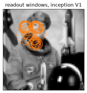
Each neuron reads the feature map through a Gaussian window. The circles are the windows of the 50 V1 neurons.

time: <1 sec

%%time

# 1. three example photos, in the canonical input format
photos = {
    "astronaut": skdata.astronaut(),
    "cat": skdata.chelsea(),
    "coffee": skdata.coffee(),
}

# [3, 1, 64, 64] in [-1, 1]
images = torch.stack([to_input(p) for p in photos.values()])
print(
    "images:",
    tuple(images.shape),
    "range",
    float(images.min()),
    "to",
    float(images.max()),
)

# 2. draw the readout windows (centre mu, width sigma) on the first photo
mu, sigma = (
    encoder.readout.mu.detach().cpu(),
    encoder.readout.sigma.detach().cpu().abs(),
)

fig, ax = plt.subplots(figsize=(3.6, 3.6))
ax.imshow(images[0, 0], cmap="gray", extent=(-1, 1, 1, -1), vmin=-1, vmax=1)
for (x, y), s in zip(mu.tolist(), sigma.tolist()):
    ax.add_patch(Circle((x, y), s, fill=False, color="tab:orange", lw=0.8))

ax.set_xlim(-1, 1)
ax.set_ylim(1, -1)
ax.set_xticks([])
ax.set_yticks([])
ax.set_title("readout windows, inception V1")
plt.show()

images: (3, 1, 64, 64) range -1.0 to 0.9843137264251709

3. Predict neural responses

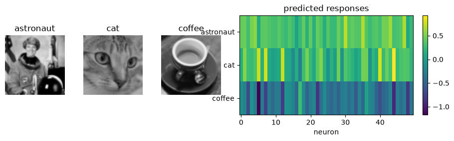
encoder.predict(images) returns one row per image and one column per neuron. Images are [N, 1, 64, 64] in [-1, 1].

time: <1 sec

%%time

# predicted responses: one row per image, one column per neuron
responses = encoder.predict(images)
print("responses:", tuple(responses.shape), "(images x neurons)")

# the images (left) and their predicted responses (right)
fig, axes = plt.subplots(
    1, 4, figsize=(11, 2.6), gridspec_kw={"width_ratios": [1, 1, 1, 3.2]}
)

for ax, (name, _), x in zip(axes, photos.items(), images):
    ax.imshow(x[0], cmap="gray", vmin=-1, vmax=1)
    ax.set_title(name)
    ax.axis("off")

im = axes[3].imshow(responses, aspect="auto", cmap="viridis")
axes[3].set_yticks(range(3))
axes[3].set_yticklabels(photos)
axes[3].set_xlabel("neuron")
axes[3].set_title("predicted responses")
fig.colorbar(im, ax=axes[3], fraction=0.04)
plt.show()

responses: (3, 50) (images x neurons)

4. Compute the Fisher information metric J(x)

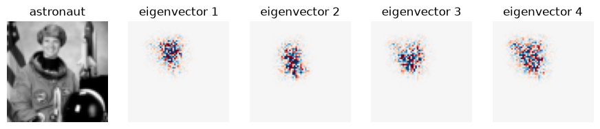
validate_encoder checks the encoder contract. compute_fisher returns the leading eigenvectors of J(x) at one image: the image changes that move the predicted responses the most.

Details

The contract is a differentiable function from an image to responses, so every tool of the package accepts the encoder. \(J(x)=\frac{1}{\sigma^2}J_f(x)^\top J_f(x)\), where \(J_f\) is the Jacobian of the responses with respect to the pixels and \(\sigma\) the noise of the neurons.

time: <1 sec

%%time

# 1. check that the encoder follows the encoder contract
report = validate_encoder(encoder, sigma=0.22)
print(
    "contract satisfied:",
    report.n_neurons,
    "neurons, response std",
    round(report.response_std, 2),
    "| warnings:",
    report.warnings or "none",
)

# 2. Fisher information J(x) at the first image: its top-4 eigenpairs
fisher = compute_fisher(
    image=images[:1], encoder=encoder, sigma=0.22, top_k=4, device=torch.device(device)
)

print("eigenvalues:", [f"{v:.3g}" for v in fisher.eigenvalues.tolist()])

# 3. the image and its leading eigenvectors
fig, axes = plt.subplots(1, 5, figsize=(11, 2.5))
axes[0].imshow(images[0, 0], cmap="gray", vmin=-1, vmax=1)
axes[0].set_title("astronaut")
for k, ax in enumerate(axes[1:]):
    v = fisher.eigenvectors[k].reshape(64, 64).cpu()
    m = v.abs().quantile(0.99)
    ax.imshow(v, cmap="RdBu_r", vmin=-m, vmax=m)
    ax.set_title(f"eigenvector {k + 1}")

for ax in axes:
    ax.axis("off")

plt.show()

contract satisfied: 50 neurons, response std 0.12 | warnings: none
eigenvalues: ['176', '115', '50.3', '35.7']

5. The other encoders of the paper

The same lines work for every checkpoint.

time: 1 sec

%%time

# the same calls work for every checkpoint of the paper
for name in ("inception", "resnet50"):
    for area in ("V1", "V4"):
        enc = load_encoder(name, area=area)
        out = enc.predict(images)
        print(
            f"{name:9s} {area}: predicts {tuple(out.shape)} | "
            f"{enc.summary().split(': ', 1)[1]}"
        )

inception V1: predicts (3, 50) | backbone InceptionBackbone (out [C=192, 12, 12]), readout GaussianReadout, 50 neurons, 9,800 trainable / 182,472 parameters
inception V4: predicts (3, 50) | backbone InceptionBackbone (out [C=192, 12, 12]), readout GaussianReadout, 50 neurons, 9,800 trainable / 182,472 parameters
resnet50  V1: predicts (3, 50) | backbone ResNet50Backbone (out [C=256, 16, 16]), readout GaussianReadout, 50 neurons, 13,000 trainable / 97,544 parameters
resnet50  V4: predicts (3, 50) | backbone ResNet50Backbone (out [C=256, 16, 16]), readout GaussianReadout, 50 neurons, 13,000 trainable / 97,544 parameters

6. Recap

To do	Call
load an encoder of the paper	load_encoder("inception", area="V1")
load a checkpoint from disk	load_encoder("path/to/encoder.pt")
predict neural responses	encoder.predict(images)
check the encoder contract	multigeom.validate_encoder(encoder)
Fisher information of one image	multigeom.compute_fisher(image=x, encoder=encoder, sigma=0.22)

Next: notebook 1 builds an encoder of your own, fits it to neural data, saves it and loads it back.