Compute G(x)#

Author: laquitainesteeve@gmail.com
Goal: Train the diffusion model that the multi-scale Fisher metric G(x) needs, with responses predicted by the encoder of notebook 1, then compute and plot G(x) and J(x). Any encoder that follows the encoder contract works.
Requirements: notebook 1 run once, TinyImageNet (downloaded on the first run), diffusers, and preferably a GPU.
Time: about 2 min on a GPU. The model is tiny, so G(x) is rough; notebook 3 shows the quality of the paper’s checkpoints.

1. Setup#

1.1. Install package#

On Google Colab, install multigeom and diffusers; elsewhere this does nothing.

time: <1 sec

[1]:

%%time

# on Google Colab install the package from PyPI, without its dependencies: Colab already
# has torch, numpy, scipy and matplotlib, and reinstalling torch is slow and can break
# the GPU runtime (nothing to do on your own machine)
import sys

if "google.colab" in sys.modules:
    %pip install -q --no-deps --pre multigeom
    %pip install -q "diffusers>=0.30,<0.38"     # the diffusion model of this notebook

CPU times: user 2 μs, sys: 0 ns, total: 2 μs
Wall time: 4.05 μs

1.2. Imports and parameters#

Work from the repository root, import the packages, set the parameters and pick the device.

time: 3 secs

[2]:

%%time

# move to the repository root (the folder containing environment.yml): data/ and runs/
# are read from there
import os
from pathlib import Path

root = Path.cwd().resolve()
while not (root / "environment.yml").exists() and root != root.parent:
    root = root.parent

if (root / "environment.yml").exists():
    os.chdir(root)

print("working folder:", Path.cwd())

# libraries and the package
import time

import matplotlib.pyplot as plt
import numpy as np
import torch

import multigeom
from multigeom import compute_fisher, compute_g, load_encoder, subspace_alignment
from multigeom.config import load_config
from multigeom.datasets import GaborTeacher, TinyImageNetDataset, download_tinyimagenet
from multigeom.diffusion import DiffusionConfig
from multigeom.diffusion.model import build_diffusion_model, build_scheduler
from multigeom.diffusion.responses import precompute_responses
from multigeom.diffusion.train import train_diffusion
from multigeom.utils import make_generator

# device and random seed
device = "cuda" if torch.cuda.is_available() else "cpu"
dev = torch.device(device)
torch.manual_seed(0)

# parameters
SAVE_DIR = Path("runs/getting_started")

# TinyImageNet images to train the diffusion model on (200 classes)
IMAGES_PER_CLASS = 100
EPOCHS = 5
N_MC = 50  # Monte-Carlo samples of the G(x) estimator (the paper uses 200)

# spacing of the diffusion times in the integral over scales (the paper uses 40)
TIMESTEP_STEP = 80
N_COMPARE = 10  # test images for the comparison with the ground truth
if device == "cpu":  # a few minutes on a CPU
    IMAGES_PER_CLASS, EPOCHS, N_MC, TIMESTEP_STEP, N_COMPARE = 10, 1, 10, 160, 3

print("multigeom", multigeom.__version__, "| device:", device)

working folder: /home/steeve/steeve/idv/code/multigeom-tutorials
multigeom 0.1.0.dev2 | device: cuda
CPU times: user 4.22 s, sys: 363 ms, total: 4.58 s
Wall time: 3.3 s

1.3. Custom functions#

show draws one eigenvector as an image.

time: <1 sec

[3]:

%%time


def show(ax, vec):
    """Draw one eigenvector as a 64 x 64 image (red positive, blue negative)."""
    v = vec.reshape(64, 64).cpu()
    m = v.abs().quantile(0.99)
    ax.imshow(v, cmap="RdBu_r", vmin=-m, vmax=m)
    ax.axis("off")

CPU times: user 3 μs, sys: 0 ns, total: 3 μs
Wall time: 6.44 μs

2. Load the encoder and predict responses to many images#

We load the encoder saved by notebook 1 (or load_encoder("inception", area="V1")). The diffusion model is trained on TinyImageNet images with the responses predicted by the encoder.

time: 4 secs

[4]:

%%time

# 1. the encoder saved by notebook 1
encoder_path = SAVE_DIR / "encoder.pt"
if not encoder_path.exists():
    raise FileNotFoundError(
        f"{encoder_path} not found: run notebook 1 first, or load an encoder of the "
        "paper: "
        "load_encoder('inception', area='V1')"
    )

encoder = load_encoder(encoder_path, device=device)
print(encoder.summary())

# 2. TinyImageNet training images
download_tinyimagenet()  # 240 MB, downloaded the first time only (about 1 min)
dataset = TinyImageNetDataset("train", images_per_class=IMAGES_PER_CLASS)

# [N, 1, 64, 64] in [-1, 1]
images = torch.stack([dataset[i] for i in range(len(dataset))])

# 3. responses predicted by the encoder: the conditioning of the diffusion model
t0 = time.time()
responses = precompute_responses(encoder, images, batch_size=512, device=device)
print(
    f"{len(images)} images -> responses {tuple(responses.shape)} in "
    f"{time.time() - t0:.1f} s; "
    f"mean {responses.mean():.2f}, std {responses.std():.2f}"
)

NeuralEncoder: backbone SmallCNNBackbone (out [C=64, 16, 16]), readout GaussianReadout, 50 neurons, 59,976 trainable / 59,976 parameters
20000 images -> responses (20000, 50) in 0.9 s; mean 1.29, std 0.64
CPU times: user 13.3 s, sys: 555 ms, total: 13.8 s
Wall time: 4.94 s

3. Set up the diffusion model#

DiffusionConfig.for_encoder(encoder) sets the conditioning width to the number of neurons. We shrink the model so that it trains in about a minute.

Details

	paper	here
UNet channels, layers per block	(64, 128, 256, 512), 2	(32, 64, 128, 128), 1
conditioning width	256	64
training images, epochs, batch	100,000, 200, 128	`IMAGES_PER_CLASS` x 200, `EPOCHS`, 64

The noise sigma of the observation model (0.22) must be the same in the diffusion model and in the estimator; both read it from the packaged configuration.

time: <1 sec

[5]:

%%time

# conditioning input width = number of neurons
cfg = DiffusionConfig.for_encoder(encoder)

# shrink the model and the recipe so that it trains in about a minute
cfg.unet.block_channels = [32, 64, 128, 128]
cfg.unet.layers_per_block = 1
cfg.unet.cross_attention_dim = 64
cfg.conditioning.mlp_layers = [encoder.n_neurons, 64, 64, 64]
cfg.train.epochs, cfg.train.batch_size, cfg.train.lr, cfg.train.warmup_steps = (
    EPOCHS,
    64,
    3e-4,
    100,
)

# build it once, to count its parameters
model = build_diffusion_model(cfg)
print(
    f"diffusion model: {sum(p.numel() for p in model.parameters()) / 1e6:.1f} M "
    "parameters "
    f"(the paper's: 68 M) | noise sigma {cfg.conditioning.observation_noise_sigma}"
)

del model

diffusion model: 5.5 M parameters (the paper's: 68 M) | noise sigma 0.22
CPU times: user 86 ms, sys: 4.33 ms, total: 90.3 ms
Wall time: 39.8 ms

4. Train the diffusion model#

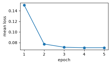
train_diffusion(cfg, images, responses, out_dir) writes final_model.pt after every epoch and resumes an interrupted run with resume=True.

Details

It trains the model to predict the noise added to the images, given the noisy responses, with classifier-free guidance dropout so that the same network also gives the unconditional prediction.

time: 2 min

[6]:

%%time

# train: the model learns to predict the noise added to the images, given the responses
t0 = time.time()
history = train_diffusion(
    cfg,
    images,
    responses,
    SAVE_DIR / "diffusion",
    device=device,
    num_workers=0,
    save_every=1000,
    log=None,
)

print(
    f"trained for {EPOCHS} epochs in {time.time() - t0:.0f} s | loss "
    f"{history['loss'][0]:.3f} -> {history['loss'][-1]:.3f}"
)

# training loss
plt.figure(figsize=(4, 2.4))
plt.plot(history["epoch"], history["loss"], "o-")
plt.xlabel("epoch")
plt.ylabel("mean loss")
plt.tight_layout()
plt.show()

trained for 5 epochs in 99 s | loss 0.151 -> 0.070

../_images/demo_notebooks_2_compute_g_13_2.png

CPU times: user 8min 2s, sys: 1.18 s, total: 8min 4s
Wall time: 1min 39s

5. Compute G(x) and J(x)#

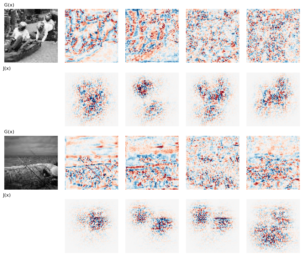
For test images the diffusion model never saw, compute_g gives the leading eigenvectors of the multi-scale Fisher metric G(x), and compute_fisher those of J(x).

Details

compute_g is the conditional-pair estimator of the paper: Monte-Carlo samples at every diffusion time, noise-prediction differences for two responses sampled around the encoder’s prediction, then an SVD. compute_fisher is closed form from the encoder’s Jacobian. Both take the image, the encoder and settings; compute_g also takes the diffusion model and its noise schedule.

time: 2 min

[7]:

%%time

# 1. the trained diffusion model and its noise schedule
unet = build_diffusion_model(cfg).to(dev)
unet.load_state_dict(
    torch.load(
        SAVE_DIR / "diffusion" / "final_model.pt", map_location=dev, weights_only=False
    )["model_state_dict"]
)

unet.eval()
alphas_cumprod = build_scheduler(cfg).alphas_cumprod.to(dev)

# 2. settings of the estimator
est = load_config("estimator")  # the packaged settings of the estimator
est.monte_carlo.n_samples = N_MC
est.monte_carlo.timestep_grid.step = TIMESTEP_STEP
est.top_k = 20
sigma = float(est.monte_carlo.observation_noise_sigma)

# 3. G(x) and J(x) for the test images
# TinyImageNet validation images
test_images = torch.stack([TinyImageNetDataset("val")[i] for i in range(N_COMPARE)])

G, J = [], []
t0 = time.time()
for i, x in enumerate(test_images):
    x = x.unsqueeze(0).to(dev)
    G.append(
        compute_g(
            image=x,
            encoder=encoder,
            unet=unet,
            alphas_cumprod=alphas_cumprod,
            cfg=est,
            device=dev,
            generator=make_generator(int(est.seed) + i, dev),
        )
    )
    J.append(
        compute_fisher(image=x, encoder=encoder, sigma=sigma, top_k=20, device=dev)
    )

print(f"G(x) and J(x) for {len(test_images)} images in {time.time() - t0:.1f} s")
print(
    "leading eigenvalues of G(x), image 0:",
    [f"{v:.3g}" for v in G[0].eigenvalues[:4].tolist()],
)

print(
    "leading eigenvalues of J(x), image 0:",
    [f"{v:.3g}" for v in J[0].eigenvalues[:4].tolist()],
)

<timed exec>:39: UserWarning: R9: responses have std 0.0705 over random test images, while the noise sigma is 0.22; the pipeline expects responses of order 1 (for example z-scored). Rescale the model's output or set sigma accordingly. (Random noise images only approximate natural-image statistics.)

G(x) and J(x) for 10 images in 116.1 s
leading eigenvalues of G(x), image 0: ['0.697', '0.121', '0.0839', '0.0639']
leading eigenvalues of J(x), image 0: ['88.7', '50.4', '39.3', '32.1']
CPU times: user 31min 4s, sys: 401 ms, total: 31min 4s
Wall time: 1min 57s

6. Plot#

The leading eigenvectors of each metric (red positive, blue negative; the sign is arbitrary), as in the paper’s Fig. 3E-F.

time: <1 sec

[8]:

%%time

# image, leading eigenvectors of G(x) (first row) and of J(x) (second row) of the first
# test images
n_show = min(2, len(test_images))
fig, axes = plt.subplots(2 * n_show, 5, figsize=(10, 4.2 * n_show))
for i in range(n_show):
    for r, (label, out) in enumerate([("G(x)", G[i]), ("J(x)", J[i])]):
        row = 2 * i + r
        axes[row, 0].imshow(
            test_images[i, 0], cmap="gray", vmin=-1, vmax=1
        ) if r == 0 else None
        axes[row, 0].axis("off")
        axes[row, 0].set_title(label, loc="left", fontsize=11)
        for k in range(4):
            show(axes[row, k + 1], out.eigenvectors[k])

plt.tight_layout()
plt.show()

../_images/demo_notebooks_2_compute_g_17_0.png

CPU times: user 270 ms, sys: 1 μs, total: 270 ms
Wall time: 259 ms

7. Compare with the ground truth#

The subspace alignment \(\mathcal{A}_k\) is 1 when the top-k eigenvectors of two metrics span the same subspace (chance: k / 4096). We compare the encoder’s G(x) and J(x) with the teacher’s J(x), averaged over test images.

Details

The diffusion model here is tiny and briefly trained, there is one fitted encoder, and the teacher’s own G(x) would need a diffusion model trained on the teacher’s responses. The numbers say how close this small experiment gets, nothing more.

time: <1 sec

[9]:

%%time

# 1. the ground-truth teacher saved by notebook 1, and its J(x) at the test images
saved = torch.load(SAVE_DIR / "teacher.pt", weights_only=False)
teacher = GaborTeacher(saved["n_neurons"], seed=saved["seed"]).to(dev)
teacher.load_state_dict(saved["state_dict"])
J_true = [
    compute_fisher(
        image=x.unsqueeze(0).to(dev), encoder=teacher, sigma=sigma, top_k=20, device=dev
    )
    for x in test_images
]

# 2. subspace alignment with the ground truth, for a few values of k
print(
    f"subspace alignment with the ground-truth J(x), mean over {len(test_images)} "
    "images (chance = k / 4096):"
)

print(f"{'k':>3s} {'chance':>8s} {'J of the encoder':>18s} {'G of the encoder':>18s}")
for k in (1, 5, 10):
    a_j = np.mean(
        [
            subspace_alignment(j.eigenvectors.cpu(), t.eigenvectors.cpu(), k)
            for j, t in zip(J, J_true)
        ]
    )
    a_g = np.mean(
        [
            subspace_alignment(g.eigenvectors.cpu(), t.eigenvectors.cpu(), k)
            for g, t in zip(G, J_true)
        ]
    )
    print(f"{k:3d} {k / 4096:8.4f} {a_j:18.3f} {a_g:18.3f}")

subspace alignment with the ground-truth J(x), mean over 10 images (chance = k / 4096):
  k   chance   J of the encoder   G of the encoder
  1   0.0002              0.009              0.009
  5   0.0012              0.011              0.011
 10   0.0024              0.016              0.014
CPU times: user 3.24 s, sys: 9.02 ms, total: 3.24 s
Wall time: 391 ms

8. Recap and next steps#

To do	Call
responses of an encoder to many images	`precompute_responses(encoder, images)`
diffusion configuration for an encoder	`DiffusionConfig.for_encoder(encoder)`
train the diffusion model	`train_diffusion(cfg, images, responses, out_dir)`
multi-scale Fisher metric G(x)	`multigeom.compute_g(image=x, encoder=encoder, unet=unet, alphas_cumprod=..., cfg=est, device=...)`
Fisher information J(x)	`multigeom.compute_fisher(image=x, encoder=encoder, sigma=0.22)`
similarity of two sets of eigenvectors	`multigeom.subspace_alignment(eigvecs_a, eigvecs_b, k)`

The same steps, for many images and several encoders, are the command-line stages of the pipeline (multigeom train-diffusion, multigeom compute-g, multigeom align). Next: notebooks 3 to 6 reproduce the figures of the paper from its trained checkpoints.